Matrix processing of Sun H-Alpha zones around sunspots.
(by Sylvain Weiller http://sweiller.free.fr )Introduction
Early 2009 is still a quiet period of the Sun
activity. But a few years ago almost every day something was happening on its
surface and every solar astrophotographer was overbooked !
H-alpha is the light band were most of the
visible activity takes place. When Coronado introduced the SolarMax HA filters series
I bought the 90mm one instead of a new car ! Nowadays almost everybody can do
H-alpha solar imaging with the cheaper PST.
All the AVIs are done with a Perl Vixen fluorite
4" refractor, the Coronado SM90 (90mm) and a Toucam Pro in RAW mode. In
general during the day, with warm air and local constructions not far from my
observatory terrace, seeing is not very good. Also very often, H-Alpha solar
AVIs cannot be stacked as a flare is going on (because every image is different) and the astronomer then
does animations ! The 1min one, at 10fps - in between flares - I propose to
process with you has been one of the most spectacular !
I am much grateful to Cor for his great software
RegiStax. Originally this AVI had been processed with Registax 4 in single
point mode. Reprocessing it with a matrix in version 5 has improved the result
quite a bit !
Loading & Alignment
Load the AVI and uncheck colour if set. Lets try
to find automatically a best frame to use as a reference frame. As the frames
are contrasted at all, set filters with stretch activated (80-250).
In standard mode, a zone with high contrast is chosen and ‘scan frames’ is hit. Scan frames will at the same time find the area common to all frames and align them by quality ! Put 100% in frame quality to see it rightaway when done.
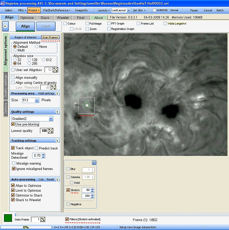 Image 1
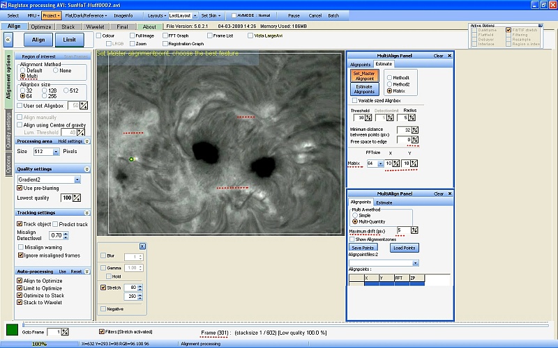
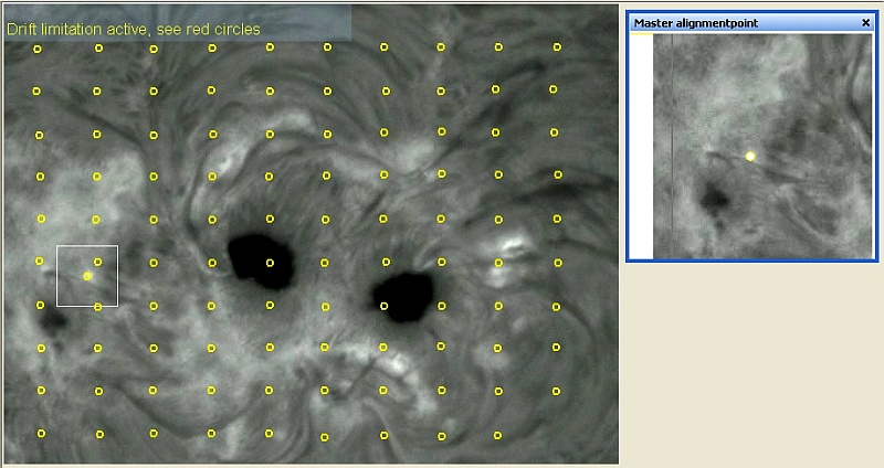
In ‘estimate’ tab, click on Set_master
Alignpoint, this sets the master Alignpoint (AP) at the previous scanframe AP.
Choose alignment method multi, with a size of 64.
Quality settings is set to Gradient2 and preblurring. As there are no
particular punctual contrasted features and a rather equal processing on all
the surface is wanted, we will work with a matrix covering the image. In ‘alignpoint’
tab (shown in this article superposed)
maximum drift is set to 5 pixels. In ‘estimate’ tab
set a 10*10 matrix. Free space to edge is set to 0.
Click on ‘estimate alignpoints’ and the matrix
is set, inside the scanframes area … Note
that in alignpoint window, it is of good practice to save the APs (‘Save
Points’) as a .rap file for later re-use.
Now ready to click on Align …
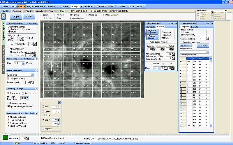
Alignpoints are slightly moving but happily their
drift is limited by our 5 pixel setting around the MasterPoint.
After a while, basic alignment is done and limit
tab bottom lights up in green.
Lowest quality value of 95% gives us 56 (not
enough to later avoid an important role of the noise after wavelets) and 90%
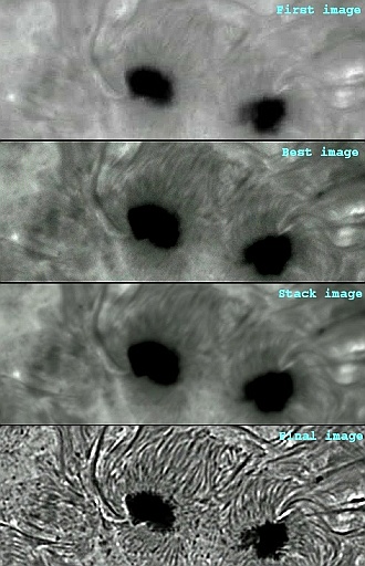
280 frames to keep. If we have a look at the best frame (301) found by RegiStax
5 we can see what kind of details we have and choose a better limit. We don’t
want to blur the fine details underlined in red ! Finally a stack of 160 is
rather good (see below) . Hit limit.
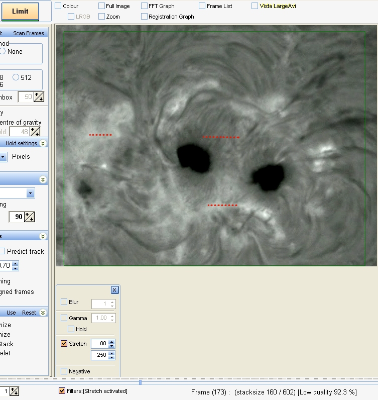
Image 5
Optimize is done in V5 style and Absolute.
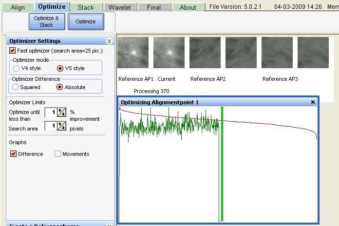 Image 6
Stack
Click on Stack tab.
Here lets show the stackgraph panel.
In the top window we eliminate the worst quality
frames. Stack is now 139.
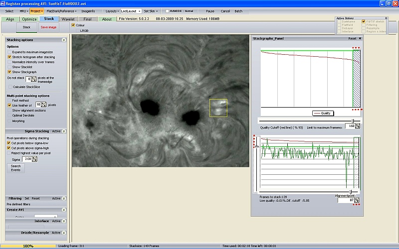
We can also act individually on all APs to eliminate frames
– especially the ones with contrasted details - with to much difference with
the average (green pics going very high) like here for PA 87 eg.
The feather options is set to 10 pixels, stretch
histogram is checked.
Click on Stack… and wait for a few minutes.
At the end of stack process, we see that now the
original 80-250 stretching is gone.
Wavelets
Lets look for eventual un-feathered lines to know
where to look later !
To do this we push the wavelet cursors of layer 1, 2,
3 to 100% foolowed by Do_all.
We can see were we need to be vigilant in the
following process.
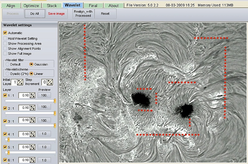
After this hit the reset (wavelet) tab above the image.
Of course here there is a lot of testing, coming backs
etc…
In the following composite image we can find some
clues …
a) It is important to lower the overall contrast of
the image (here 75%).
b) In wavelet settings : Automatic is checked.
Wavelet filter is set to Gaussian-Linear with a step increment is set to 1
(instead of normal 0) as this leads to less visible spurious un-feathered
lines. Layer 1 is unchecked as it is the most noisy. Layer 2 is at middle
range.
c) Create_Mask_Panel is used in Low_High_Clipping
mode. The position of the cursor gives the effects shown in Compare.
d) In top Compare we see that the bottom zoomed
image of the sunspot has a more natural looking especially near the edges and
the difference – in colors - of the 2 images. In bottom (glued here from
another printscreen) Compare we see
that we avoid saturation and get more details in the brightest zones.
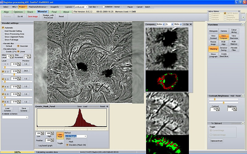
After all this work hit Do_All and lets go to the
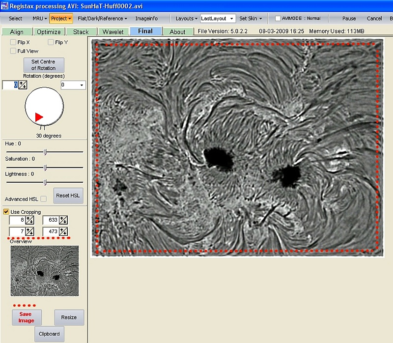
final page to cut the unwanted borders before saving the final image.
Conclusion :
Lets summarize the processing with a comparison
image !
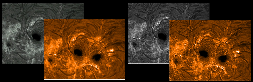
And finally the series that shows the differences between the original image and the final image.
For
more examples visit http://sweiller.free.fr